Close
In the following exercise, we will practice writing an automation script to calculate liquidity ratios. This script will also create an MS Excel file containing the results and three graphs so that we can visualize the liquidity ratios.
The objective of this exercise is to practice working with real-world data and to see how automation can help you be more productive.
You can also read the article "How to use a python custom module to simplify your work" to learn more about the python module used in this exercise.
We want to automate the creation of a worksheet that contains a table with three liquidity ratios for Apple Inc. for the last 10 years. We also want to visualize the liquidity ratios while comparing them with industry ratios when possible.
The liquidity ratios that we want to calculate:
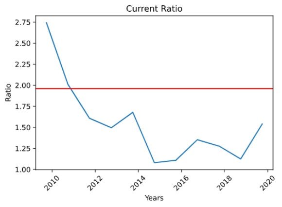
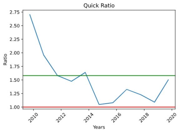
According to Guru Focus, as of 8-10-2020, the industry liquidity ratios are 1.96 for the Current Ratio and 1.58 for the Quick Ratio. There is no industry ratio for the Cash Ratio, so we will need to compare it with the results from previous years.
The following resources are made available to us for this exercise:
apple.csv, which contains the last ten years of Apple Inc.'s annual accounting data for the following balance sheet accounts:financialratios.py. This file is the custom python module that stores the functions needed to calculate each ratio.Both files and a copy of the final python script are available from the project repository. You can also get the complete financial information of Apple Inc. here.
Additionally, you will also need to have installed Python 3.8 on your computer with the following libraries:
Finally, you will need a code editor. I will be using Microsoft Visual Code as my code editor.
The instructions for this exercise are as follows:
apple.csv and financialratios.py files from the project repository.df.df_ratios to store Apple Inc.'s liquidity ratiosdf_ratios DataFrame.Liquidity ratios are metrics used to measure a company's ability to meet its short-term obligation or liabilities. The two most common liquidity ratios used in financial analysis are the current ratio and the quick ratio. You can learn more about financial ratios by reading the article "What are Financial Ratios?" by the Corporate Finance Institute or any Financial Management textbook.
The following steps can be followed to writing the script about liquidity ratios:
Before we begin to write the Python script, download the exercise files apple.csv and the python module financialratios.py. Save both files to the project's folder.
Next, open your code editor of choice and create the file for the script in the project's folder where you have stored the apple.csv and the financialratios.py module.
With everything setup, we can now start writing the script.
The first step is to import the necessary python module and libraries.
from matplotlib.pyplot import colorbar
import financialratios as fr
import pandas as pd
import matplotlib.pyplot as plt
apple.csv fileOur third step is to import the data stores in the file apple.csv. We will import the data into a panda's DataFrame object called df.
df = pd.read_csv('apple.csv', index_col='Date', parse_dates=True)
Because the apple.csv the file also contains dates; we can also set the column "Date" as our index. We can parse the content in the "Date" column as a datetime datatype.
Now that we have imported our data and saved it to the DataFrame df, we can create the empty DataFrame where we want to store the results. We can call this DataFrame df_ratios by writing the following code:
# Create the column names
column_names = ["Current Ratio", "Quick Ratio", "Cash Ratio"]
# Create the empty dataframe
df_ratios = pd.DataFrame(columns=column_names)
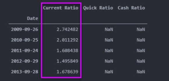
Our fifth step is to use the custom module financialratios to call the function get_current_ratio and calculate the current ratio. We will store the results into the new DataFrame df_ratios under the column named "Current Ratio". Here is the line of code we need to write:
df_ratios["Current Ratio"] = fr.get_current_ratio(df['current assets'], df['current liabilities'])
Let us dig down to see what we just wrote:
Current Ratio of the DataFrame df_ratios .get_current_ratio from the custom module that we imported and named fr.df.df.We can check that the calculation has been done correctly by calling the .head method on df_ratios by printing df_ratios.head()
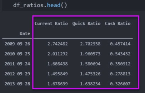
Now that we know our script is working, we can continue calculating the other two ratios in the same way we did with the current ratio.
df_ratios["Quick Ratio"] = fr.get_quick_ratio(df['current assets'], df['inventories'], df['current liabilities'])
df_ratios["Cash Ratio"] =  fr.get_cash_ratio(df['cash & cash equivalent'], df['current liabilities'])
We can check that the calculations have been done correctly by calling the .head method on df_ratios.
Now that we have calculated all the liquidity ratios for the last ten years, we can export the table to a Microsoft Excel file. We can export the results by writing the following line of code.
df_ratios.to_excel('liquidity-ratios.xlsx')
As we can see in our folder, the liquidity-ratios.xlsx file has been created and can now be open using Microsoft Excel.
In this step, we will use the library matplotlib to plot the current ratios for the past 10 years. Remember that we will set the industry average at 1.96.
plt.plot(df_ratios['Current Ratio'])
plt.axhline(y=1.96, color='r')
plt.xticks(rotation=45)
plt.title('Current Ratio')
plt.xlabel('Years')
plt.ylabel('Ratio')
plt.show()
If we run the script we get the following graph:
Next, we will visualize the quick ratio, setting the industry ratio to 1.58.
plt.plot(df_ratios['Quick Ratio'])
plt.axhline(y=1.58, color='g')
plt.axhline(y=1, color='r')
plt.xticks(rotation=45)
plt.title('Quick Ratio')
plt.xlabel('Years')
plt.ylabel('Ratio')
plt.show()
If we run the script we get the following graph:
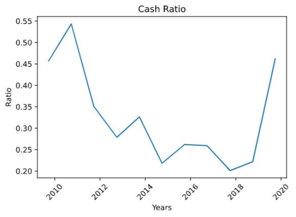
The last step to be included in the script is the lines of code that will allow us to visualize Apple's cash ratio for the last 10 years.
plt.plot(df_ratios['Cash Ratio'])
plt.xticks(rotation=45)
plt.title('Cash Ratio')
plt.xlabel('Years')
plt.ylabel('Ratio')
plt.show()
If we run the script we get the following graph:
I hope you found this project useful and that you now have a better understanding of how python can be of great tool to use for automating repetitive tasks like calculating financial ratios. Moreover, I hope you can apply what you have learned in your job. Remember that you can extend the script you just wrote to calculate other ratios. You can also modify the python module to included different ratios too.
Please feel free to share this article with your coworkers, friends, and family through social media. You can also subscribe to my mailing list to receive information when I publishing new content.
Again thank you for taking the time to read this article.
